The Heartbeat of the Market: A Friendly Guide to Implied and Local Volatility

This blog post explains why the standard “speed limit” (Black-Scholes) fails to predict market crashes, leading to the “Volatility Smirk” driven by investor fear. It clarifies the difference between Implied Volatility (your average trip speed) and Local Volatility (your speedometer’s exact wiggle at a specific price), stripping away the math jargon to reveal the human story of risk behind the formulas.

Introduction

If you’ve ever looked at an options chain, you’ve seen a number called Implied Volatility (IV). To most, it’s just a percentage, but to a quant, it is the “DNA” of market sentiment. Understanding the difference between Implied Volatility and its cousin, Local Volatility, is like the difference between a weather forecast and the actual rain falling on your head.

1. Implied Volatility: The “Market’s Guess”

Think of Implied Volatility as the speed limit the market expects a stock to travel at over a certain period. This answers the question what single volatility number for a strike K with maturity T is best if the option is held till maturity.

The Analogy:

Imagine you are buying insurance for a teenager’s car. The insurance company doesn’t know exactly how the teen will drive, so they look at the “market price” of accidents and work backward to figure out the risk.

The Simple Logic: In the Black-Scholes model, we have a “pricing machine.” You put in the stock price (S), strike (K), time (T), and interest rate (r). Normally, you’d add volatility $\sigma$ to get a price. But in the real world, we already have the price $(C_{mkt})$ from the exchange.

$C_{BS}(S, K, T, r, \sigma_{impl}) = C_{mkt}$

Implied Volatility is simply the value of $\sigma$ that makes the math match the market reality.

2. The Mystery of the “Smirk”

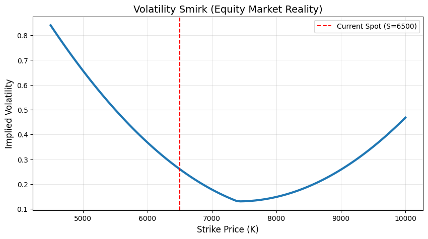
If the Black-Scholes model were perfect, IV would be a flat line. Whether you bought a strike at $5,000 or $10,000, the “expected speed” of the stock should be the same.

But as we see in our diagram, it looks like a Smirk.

Why? Investors have “Crashphobia.” They are terrified of a sudden drop, so they bid up the price of low-strike puts.
The Result: To justify those high prices, the “pricing machine” has to spit out a higher IV for lower strikes.

3. Local Volatility: The “Instantaneous Truth”

While Implied Volatility is an average over the life of the option, Local Volatility is the volatility at a specific point in time and at a specific stock price.

This answers the question what is the instantaneous volatility of the stock price at that exact moment t and price level S.

It can be considered as the volatility of the stock at price S and time t that explains all these different option prices at once.

The Analogy:

Implied Volatility is your average speed over a 4-hour road trip (e.g., 60 mph).
Local Volatility is your speedometer reading at exactly 2:15 PM while driving through a specific school zone (e.g., 20 mph).

The Intuition: Local Volatility (often associated with the Dupire Formula) asks: “If the stock hits $7,000 in exactly 3 months, how much will it be wiggling at that exact moment?”

The Dupires Formula is as follows.

\sigma_{loc}^2(K, T) = \frac{\frac{\partial C}{\partial T} + rK \frac{\partial C}{\partial K}}{\frac{1}{2}K^2 \frac{\partial^2 C}{\partial K^2}}

4. A Simple Derivation: Why Vega is Your Friend

To find these volatilities, we rely on Vega ( $\nu$ ), which measures how much an option price changes when volatility moves.

The Derivation (Simplified): We want to show that if volatility goes up, the price goes up ( $\frac{\partial C}{\partial \sigma} > 0$ ).

Start with the Call price: $C = S \Phi(d_1) - K e^{-rT} \Phi(d_2)$ .
Differentiate with respect to $\sigma$ .
After some fancy footwork with the Normal Distribution PDF ( $\phi$ ), we get: $\text{Vega} = S \phi(d_1) \sqrt{T}$

The Example: If your SPX option has a Vega of 10, and the IV jumps from 15% to 16% (a 1-point move), your option price will increase by $10. Because S, $\phi(d_1)$ , and $\sqrt{T}$ are all positive numbers, Vega is always positive. This is why your Newton-Raphson solver works so well—the price only moves in one direction relative to vol!

Feature	Implied Volatility (IV)	Local Volatility (LV)
Perspective	Forward-looking average.	Instantaneous/Spot-dependent.
Input	Market Prices ( $C_{mkt}$ ).	The entire IV Surface.
Use Case	Trading and quoting options.	Pricing exotic options (like Barriers).
Visual	The “Smile” or “Smirk”.	A complex “Terrain” or “Map”.

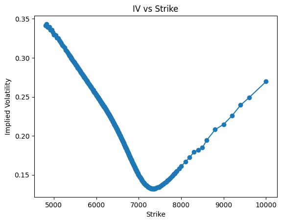
Case Study: The S&P 500 “Fear Map”

To see these concepts in action, we can look at real market data from the S&P 500 (SPX) for options expiring in June 2026. You can access the data through the CBOE website.

By taking the market’s mid-point prices and “inverting” them through our Black-Scholes solver, we reveal a striking “Volatility Smirk” that tells the story of current market sentiment.

The Setup

Current Index Level (S): ~6,582.69
Time to Expiration (T): ~0.205 years
Risk-Free Rate (r): 3.7%

The Findings: A Tale of Two Wings

When we plot the Implied Volatility (IV) against the Strike Price (K), we don’t see the flat line that classic theory predicts. Instead, we see a lopsided “U” shape:

The Left Wing (High Fear): At a low strike of 5,000, the implied volatility is a massive 34%. This represents “Crashphobia” investors are so afraid of a market collapse that they bid up the price of these “insurance” puts, forcing the implied volatility higher to match those expensive market prices.
The Bottom (Relative Calm): The lowest volatility point the “dip” in our smirk isn’t actually at the current stock price (6,582). Instead, it sits further to the right near a strike of 7,400, where IV drops to its minimum of roughly 13%. This suggests that the market currently feels most “certain” about prices slightly above the current spot level.
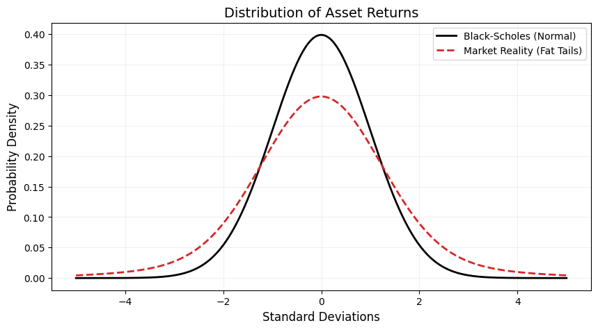
The Right Wing (Upside Uncertainty): As we move toward a high strike of 10,000, the IV climbs back up to approximately 27%. While not as extreme as the “crash” side, this reflects a demand for “lottery ticket” upside calls and the market’s acknowledgment that extreme rallies are also more likely than a standard normal distribution would suggest.

Why This Matters

This data proves that the Black-Scholes-Merton model has a fundamental weakness: it assumes volatility is constant. Our SPX plot shows that volatility is actually a “surface” that changes based on how much protection (or profit) investors are seeking at different price levels.

In short, Implied Volatility isn’t just a math input; it’s a living, breathing map of investor psychology

Final Thought: The next time you see that “Smirk” in your code, remember: you aren’t just looking at a math error in Black-Scholes. You are looking at the collective fear and insurance-buying habits of the entire world.