In Part 1, we covered what a Markov chain is, what makes a Hidden Markov Model “hidden,” and the three classic problems (Evaluation, Decoding, Learning) every HMM implementation needs to solve. In this post, we’ll build on that foundation to look at why the basic, first-order HMM can fall short for something like financial markets — and end with a small, runnable example so you can see an HMM discover hidden regimes for yourself.
The Limitation of First-Order HMMs in Finance
A first-order HMM assumes that tomorrow’s hidden state depends only on today’s hidden state — not on anything further back. But financial markets don’t always behave this way. A regime shift might build up over several days or weeks rather than being triggered by yesterday alone — think of a slow rotation from a bull market into a choppy, uncertain period, where the momentum driving that shift is spread across many past days, not just the most recent one.
If the true underlying dynamics have this kind of longer memory, a strictly one-step-back model is too restrictive to capture it. This motivates a natural question: what if the next hidden state could depend on the last n states instead of just 1?
What Are Higher-Order HMMs?
A higher-order HMM redefines the two core assumptions from Part 1:
- State transition: now conditioned on the last n states, not just the immediately preceding one: P( | )
- Emission probability: now depends on the last m hidden states, not just the current one.
Note: if n = m = 1, this collapses back to the ordinary first-order HMM from Part 1 — so first-order isn’t a fundamentally different model, just a special case of this more general one.
The catch: this blows up the parameter space significantly. For N hidden states and order n, the transition probabilities need an entry for every combination of n prior states — that’s Nn rows instead of N. Even a modest jump, like going from order 1 to order 2 with just 4 hidden states, takes you from 4 transition rows to 16. This combinatorial blowup is the practical obstacle that makes higher-order HMMs harder to train directly.
Solving this parameter explosion is possible with some clever reformulation tricks.
How Higher-Order HMMs Are Usually Solved
The core problem, again, is that a higher-order HMM’s transition probabilities blow up combinatorially — for N hidden states and order n, you need Nn rows instead of N. Rather than inventing entirely new algorithms to handle this larger space directly, the standard trick is surprisingly simple in spirit: turn the high-order problem back into a first-order one.
Here’s the idea. Instead of treating a single time step’s hidden state as the “state,” define a new super-state that bundles together a short window of consecutive hidden states — say, the current state and the previous n−1 states. So instead of asking “what’s the state at time t?”, you ask “what’s the combination of states at times t, t−1, …, t−n+1?”
Once you do this relabeling, something convenient happens: the sequence of these super-states behaves like an ordinary first-order Markov chain again. Why? Because knowing the full super-state at time t−1 (which already encodes the last n−1 individual states) is enough to determine the transition probabilities to the next super-state — you don’t need to look back any further than one step, since all the “memory” is now baked directly into the super-state itself.
The practical payoff is significant: once the problem is reframed this way, you can reuse all the standard first-order machinery — Baum-Welch for training, Viterbi for decoding, the Forward algorithm for evaluation — with no modification to the underlying algorithms. The only real cost is that your state space is larger (since each super-state represents a combination of individual states), but the math stays exactly the same as everything covered in Part 1.
This general strategy — folding a window of history into an expanded “state” so you can fall back on standard first-order tools — comes up again and again outside HMMs too. It’s the same basic idea behind, for example, turning an nth-order autoregressive time series model into a first-order vector process by stacking lagged values together.
The specific mechanics of how you construct these super-states (and how you convert model outputs back into the original, interpretable hidden states afterward) is implementation-specific — that’s exactly where we’ll go deep when we replicate the paper’s actual approach in the next project post.
Seeing It in Action: A Minimal Working Example
Theory is easier to trust once you’ve seen it work. Below is a small, self-contained example using hmmlearn (Python’s standard HMM library). We’ll simulate a simple two-regime “stock” — one calm and drifting slightly up, one volatile and drifting slightly down — and see whether a first-order Gaussian HMM can recover those regimes without ever being told they exist.
python
import numpy as np
from hmmlearn.hmm import GaussianHMM
import matplotlib.pyplot as plt

np.random.seed(42)

# Simulate a synthetic return series with 2 underlying regimes:
# regime 0 = calm, drifting slightly up
# regime 1 = volatile, drifting slightly down
n_days = 500
returns = []
state = 0
for _ in range(n_days):
    if np.random.rand() < 0.02:   # small chance of a regime switch each day
        state = 1 - state
    r = np.random.normal(0.001, 0.01) if state == 0 else np.random.normal(-0.001, 0.03)
    returns.append(r)

returns = np.array(returns).reshape(-1, 1)
prices = 100 * np.exp(np.cumsum(returns))  # convert returns to a price path

# Fit a first-order Gaussian HMM with 2 hidden states
model = GaussianHMM(n_components=2, covariance_type="diag", n_iter=1000, random_state=42)
model.fit(returns)

# Decode the most likely hidden state sequence (Viterbi under the hood)
hidden_states = model.predict(returns)

# Plot the price path, colored by which hidden state the model inferred
plt.figure(figsize=(10, 4))
for s in np.unique(hidden_states):
    mask = hidden_states == s
    plt.plot(np.where(mask)[0], prices[mask], '.', label=f"Hidden state {s}")
plt.title("Simulated Price Path Colored by Inferred Hidden State")
plt.xlabel("Day")
plt.ylabel("Price")
plt.legend()
plt.tight_layout()
plt.show()Running this, the model — with no labels, no hints about “calm” or “volatile,” nothing but the raw sequence of daily returns — cleanly separates the two regimes on its own. In this simulation, it correctly recovers the true hidden regime for about 97–98% of days.
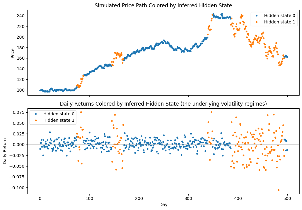
This is the payoff of the whole HMM framework: you hand it observations, and Baum-Welch (Learning) and Viterbi (Decoding) work together to uncover a latent structure you never explicitly told it about. That’s what makes HMMs appealing for financial time series in the first place — real markets don’t announce their regimes, but if regimes exist, an HMM gives you a principled way to try to recover them from price behavior alone.
Wrapping Up Parts 1 and 2
Across these two posts, we’ve built up the full picture step by step: what a Markov chain is, what changes when you add a hidden layer, the three classic problems every HMM needs to solve, and why financial time series might need more memory than a single-step model can offer — along with the general trick (folding history into an expanded “super-state”) that makes higher-order models tractable using the exact same tools.
The synthetic example above is deliberately simple — two regimes, one feature, made-up data — precisely so the underlying mechanics stay visible. Real markets are messier: returns aren’t perfectly Gaussian, regimes aren’t as clean-cut, and a single feature rarely tells the whole story.
That’s where we’re headed next. In the next post, I’ll replicate a real academic paper’s approach to this exact problem: a high-order HMM trained on real stock index data, using Gaussian mixture emissions to handle the skew and fat tails real returns actually have, and evaluated the way a quant would — with win rate, Sharpe ratio, and maximum drawdown, not just how often it “gets the regime right.” That project will also be where the higher-order mechanics from this post get implemented for real, instead of just described.