Long-Horizon Returns: Why Five-Year “Anomalies” Are So Fragile

Part 3 of my notes on empirical asset pricing

The question

Do firms that issue stock, go public, or buy other companies underperform for years afterward? Early studies said yes, dramatically. Loughran & Ritter (1995) found five-year buy-and-hold returns about 59% below comparable firms for seasoned equity offerings (SEOs) and 51% below for IPOs. Taken at face value, that means investors are badly fooled for years.

Post #1 warned that over long horizons, the model is everything. This post shows that warning playing out.

Method 1: Buy-and-hold abnormal returns (BHAR)

The intuitive approach is to buy the event firm and a matched “control” firm, hold both for five years, and compare: $BHAR_i = \prod_{t=1}^{60}(1+r_{it}) - \prod_{t=1}^{60}(1+r_{mt})$

Here $r_{mt}$ is the return on a control firm, usually matched on size and book-to-market at the time of the event.

A closely related measure is the wealth relative, the ratio instead of the difference: 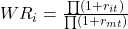$WR_i = \frac{\prod(1+r_{it})}{\prod(1+r_{mt})}$

A WR of 0.85 means $1 in the event firm grew to 85% of what $1 in the control firm grew to.

Why people like it: it matches what an investor actually experiences.

Why it’s fragile:

Compounding magnifies small errors. A benchmark that’s off by 0.3% a month becomes roughly 17% over five years. Fama (1998) and Mitchell & Stafford (2000) both stress this. Given the return is calculated by multiplying, if one wild month exists, the benchmark will be off by a lot.
The distribution is ugly. Bessembinder & Zhang (2013) report five-year BHARs for merger bidders with skewness near 29 and kurtosis over 1,400. A few extreme winners dominate, and standard t-tests become unreliable.
Matches drift apart. A control firm that looks similar on day 0 may look nothing like the event firm three years later.
Matching on two characteristics isn’t enough. This is the key point, covered below.

Method 2: Calendar-time portfolios

The main alternative flips the perspective. Each month, form a portfolio of all firms that had the event in the past 60 months. Then regress that portfolio’s monthly excess return on factors: $R_{pt} - R_{ft} = \alpha + \beta\,MKT_t + s\,SMB_t + h\,HML_t + u\,UMD_t + \varepsilon_t$

The intercept $\alpha$ is the average monthly abnormal return. It’s a single time series, so cross-firm correlation is handled automatically.

Its weaknesses:

Low power when events cluster (Loughran & Ritter, 2000). IPOs come in waves. Weighting every month equally gives a hot IPO month the same weight as a quiet one.
It can be misspecified in non-random samples (Lyon, Barber & Tsai, 1999).
It isn’t what an investor holds. The portfolio is rebalanced monthly, not bought and held.

The puzzle: the two methods disagree

To see why these two approaches disagree, think of it in terms of testing whether a new running shoe actually makes runners faster over long distances:

BHAR is like running side-by-side 5-year marathons:
- How it works: Whenever a runner buys the special shoes (the event), you find a “twin” runner of the same age, weight, and build wearing regular shoes (the matched control). Both start running, and you check back 5 years later to see the difference in total distance covered.
- The intuition: This mirrors what an individual runner actually experiences from start to finish.
- The catch: Over 5 years, life happens. One runner might twist an ankle or get sick, their fitness levels drift apart, and compounding tiny pacing differences over thousands of miles blows small measurement errors into giant gaps. A few ultra-marathoners will also skew the entire average.
Calendar-time portfolios are like monitoring a communal training track every month:
- How it works: Instead of tracking separate pairs across years, you set up a camera on a local running track. Every month, you invite anyone who bought the shoes in the last 5 years to run together as a club. You measure the club’s average monthly speed, subtract out general track conditions (weather, terrain, wind via risk factor models), and check if the shoe club consistently beats the benchmark (a club that doesn’t where the shoes, in finance it can be the Fama 5 factor or 3 factor model) month after month.
- The intuition: It avoids tracking drifting pairs and automatically averages out individual runner quirks each month. Because we are never comparing two runners, we are comparing an entire group whose idiosyncratic errors cancels each other off.
- The catch: No single runner actually trains like this (the group changes every single month), and if 100 runners bought shoes during a summer promotion and only 2 bought them in winter, looking at each calendar month with equal importance dilutes the big wave.

Here’s the tension. Eckbo, Masulis & Norli (2007) find five-year BHARs of −29.7% for SEOs and −18.0% for IPOs, both significant. For the same samples, calendar-time alphas are small and insignificant. Same firms, same period, opposite conclusions. One method must be mismeasuring “normal.”

The fix: Bessembinder & Zhang (2013)

Their diagnosis is that the control firms are imperfect matches. Event firms match their controls on size and book-to-market, but they differ systematically on five other characteristics known to predict returns across all stocks:

Characteristic	Event firms tend to have…	Known return pattern
Idiosyncratic volatility	Higher	High volatility → lower returns (Ang et al., 2006)
Illiquidity	Lower (more liquid)	More liquid → lower returns (Amihud, 2002)
Investment	Higher	High investment → lower returns (Cooper et al., 2008)
Momentum	Higher before the event	Winners keep winning in the short run (Jegadeesh & Titman, 1993)
Market beta	Higher	—

Every single row pushes event-firm returns down relative to controls for reasons that have nothing to do with issuing stock or completing a merger.

The Runner’s Handicap Analogy

Think of it like testing whether a new running shoe (the corporate event) makes runners slower over a 5-year period. You match your test runner with a “twin” runner wearing ordinary shoes, matched strictly on height and weight (size and book-to-market).

However, your test runner also happens to have a much higher resting heart rate, trains twice as hard, and runs into persistent head winds on loose gravel (volatility, investment, and liquidity biases). When your runner finishes behind their twin month after month, was it caused by the shoes, or did unmeasured physical handicaps slow them down?

Rather than combing through thousands of stocks to find a fantasy twin that matches on all seven dimensions at once—an impossible task that yields terrible matches—Bessembinder & Zhang keep the simple size and book-to-market control firm, and use regression math to purge the handicap imbalances.

How the Monthly Test Works in Practice

Instead of rolling 60 monthly returns into one giant five-year compounded number at the finish line, they structure the empirical test into firm-month observations.

If Firm A goes public and trades for 60 months, it generates 60 separate monthly rows in the dataset. If 1,000 firms go public over your sample period, that creates roughly 60,000 firm-month observations.

For every event firm i and its control twin c in each active month t, they run the regression:

$(r_{it} - r_{ct}) = a + b_1*(gap_{volatility}) + b_2*(gap_{investment}) + b_3*(gap_{momentum}) + ... + e_{it}$

The Dependent Variable ( $r_{it} - r_{ct}$ ): The difference in monthly log returns between the event firm and its size/BM control twin in month t.
The Characteristic Gaps: Each term measures the difference in a trait between the event firm and its twin in that exact month, rank-normalized between -1 and 1 so the slopes are directly comparable.
The Slopes ( $b_k$ ): Tell you exactly how much of the monthly return spread is explained simply because the two firms differ in volatility, asset growth, or momentum.
The Intercept (a): The core deliverable. It is the expected monthly return gap when every single characteristic difference equals zero. That represents the pure abnormal return attributable strictly to the corporate event.

Two Crucial Methodological Fixes

Log returns tame the skewness monster: Compounding 60 monthly simple returns into a single 5-year BHAR causes positive outliers to explode, producing skewness near 29 and kurtosis over 1,400, which wrecks standard t-tests. Bessembinder & Zhang evaluate monthly log return differences: $ln(1 + R_{it}) - ln(1 + R_{ct})$ . Log differences are additive across time and approximately symmetric, collapsing skewness down to -0.2 and making standard statistical inference reliable again.
Monthly updating solves the drifting-match trap: In a classic 5-year BHAR, a control firm chosen on Day 0 might pivot, shrink, or change capital structure by Year 3, leaving you comparing apples to oranges. In this panel setup, every characteristic gap is recalculated and updated month by month. If the control twin drifts away in risk profile over time, the monthly regression slopes absorb that drift on the fly.

The results

Event	Size/BM matching only	Plus all characteristics (with squared terms)
SEOs	−0.28%/month (WR ≈ 0.85)	≈ 0 (WR ≈ 1.00)
IPOs	−1.15%/month (WR ≈ 0.50)	−0.10%, insignificant
Merger bidders	−0.46%/month (WR ≈ 0.76)	−0.02%, insignificant
Dividend initiators	+0.40%/month (WR ≈ 1.27)	Insignificant

For SEOs, idiosyncratic volatility or investment alone removes about half of the gap. For the other events, the anomaly disappears only once nonlinear (squared) terms are included.

The calendar-time alphas in their sample are all insignificant too. Once matching is fixed, the two methods agree.

What this does and doesn’t show

It does not prove markets are efficient. The explanation relies on patterns like the volatility and momentum effects, which are themselves not fully understood. What it shows is narrower but important: these long-run returns aren’t special to the events. An IPO firm underperforms because it looks like other stocks that underperform: volatile, liquid, investing heavily. Nothing about going public is needed to explain it.

That’s the joint-hypothesis problem from post #1, resolved in favor of “bad benchmark.”

My checklist for long-horizon claims

What were the control firms matched on? Only size and B/M is a warning sign.
Do event and control firms differ on volatility, liquidity, investment or momentum?
Does the result survive both BHARs and calendar-time portfolios?
Are the returns logged, or are compounded simple returns driving the result?
Is the sample dominated by a few event waves?

Next post: portfolio sorts. How univariate, double and triple sorts work, why NYSE breakpoints matter, and how Jegadeesh & Titman built momentum portfolios.

References

Amihud, Y. (2002). Illiquidity and stock returns: Cross-section and time-series effects. Journal of Financial Markets, 5, 31–56.

Ang, A., Hodrick, R., Xing, Y., & Zhang, X. (2006). The cross-section of volatility and expected returns. Journal of Finance, 61, 259–299.

Bessembinder, H., & Zhang, F. (2013). Firm characteristics and long-run stock returns after corporate events. Journal of Financial Economics, 109(1), 83–102. https://doi.org/10.1016/j.jfineco.2013.02.009

Carhart, M. (1997). On persistence in mutual fund performance. Journal of Finance, 52, 57–82.

Cooper, M., Gulen, H., & Schill, M. (2008). Asset growth and the cross-section of stock returns. Journal of Finance, 63, 1609–1651.

Eckbo, B. E., Masulis, R., & Norli, Ø. (2007). Security offerings. In B. E. Eckbo (Ed.), Handbook of Corporate Finance: Empirical Corporate Finance, Vol. I (pp. 233–373). Elsevier/North-Holland.

Fama, E. F. (1998). Market efficiency, long-term returns, and behavioral finance. Journal of Financial Economics, 49, 283–306.

Jegadeesh, N., & Titman, S. (1993). Returns to buying winners and selling losers: Implications for stock market efficiency. Journal of Finance, 48, 65–91.

Loughran, T., & Ritter, J. (1995). The new issues puzzle. Journal of Finance, 50, 23–51.

Loughran, T., & Ritter, J. (2000). Uniformly least powerful tests of market efficiency. Journal of Financial Economics, 55, 361–389.

Lyon, J., Barber, B., & Tsai, C. (1999). Improved methods for tests of long-run abnormal stock returns. Journal of Finance, 54, 165–201.

Mitchell, M., & Stafford, E. (2000). Managerial decisions and long-term stock price performance. Journal of Business, 73, 287–329.